Graphing logarithmic functions is a fundamental skill in algebra and pre-calculus, yet many students find it intimidating because these functions behave quite differently from the linear or quadratic equations they are used to. At its core, how to graph log functions involves understanding the relationship between logarithms and exponents, as logarithms are simply the inverses of exponential functions. Once you grasp the basic shape and the role of transformations, sketching these curves becomes a predictable and systematic process. Whether you are dealing with a simple natural log or a complex transformation, mastering this skill opens the door to understanding phenomena that grow or decay at varying rates, such as sound intensity, acidity (pH levels), and seismic activity.
Understanding the Parent Logarithmic Function
Before diving into complex graphs, you must understand the parent function: f(x) = logb(x), where b > 0 and b ≠ 1. Every standard logarithmic graph shares specific characteristics that serve as your anchor points. Recognizing these features is the first step in learning how to graph log functions accurately.
- The Domain: Logarithmic functions are only defined for positive values of x. Therefore, x > 0.
- The Range: The graph extends infinitely downward and upward, meaning the range is all real numbers.
- The Vertical Asymptote: There is a vertical asymptote at x = 0 (the y-axis). The graph will get closer and closer to this line but never actually touch it.
- The X-intercept: The graph always passes through the point (1, 0) because any base raised to the power of 0 equals 1.
If the base b is greater than 1, the graph is an increasing curve. If the base b is between 0 and 1, the graph is a decreasing curve, reflecting over the x-axis.
The General Form of Logarithmic Equations
To graph more advanced equations, you need to understand how the function f(x) = a logb(x - h) + k behaves. Each constant in this formula shifts or stretches the parent graph in specific ways. Learning these transformations is the secret to knowing how to graph log functions quickly without plotting dozens of individual points.
| Constant | Transformation Effect |
|---|---|
| a | Vertical stretch (if |a| > 1) or compression (if 0 < |a| < 1); reflection over x-axis if negative. |
| h | Horizontal shift. (x - h) shifts the graph right by h units; (x + h) shifts it left. |
| k | Vertical shift. +k moves the graph up; -k moves the graph down. |
Step-by-Step Guide to Graphing
When you are faced with a new equation, following a consistent workflow will prevent errors. If you follow this logical order, you will find that graphing becomes a repeatable process.
- Identify the Vertical Asymptote: Find the value that makes the argument of the log zero. If your function is log(x - 3), set x - 3 = 0. Your vertical asymptote is x = 3.
- Determine the Key Point: For a parent function, the key point is usually (1, 0). However, due to horizontal shifts, this point moves. Find the point where the log argument equals 1. For log(x - 3), set x - 3 = 1, which gives x = 4. So, the new point is (4, 0) plus any vertical shift k.
- Find One or Two Additional Points: Plug in an easy value for x to get a secondary coordinate. For log2(x - 3), picking x = 5 makes the argument 2, and log2(2) = 1.
- Sketch the Curve: Draw your dashed line for the asymptote first. Then, plot your key points and connect them with a smooth, sweeping curve that hugs the asymptote.
💡 Note: Always double-check your horizontal shift. A common mistake is to shift in the wrong direction; remember that x - h moves to the right, while x + h moves to the left.
Advanced Considerations and Log Base Changes
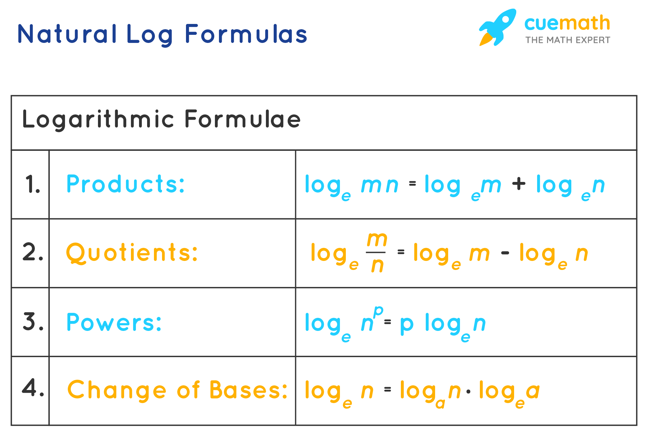
Sometimes you may encounter a base that is not convenient to calculate, such as log3(x). In these cases, you can use the Change of Base Formula: logb(x) = ln(x) / ln(b). This allows you to use a standard calculator to find coordinates for your graph. Furthermore, if you are graphing a natural logarithm ln(x), the process is identical; the only difference is that the base is the constant e (approximately 2.718).
When graphing, ensure that your scale is consistent on both the x and y axes. If you are drawing by hand, using graph paper is highly recommended. Because logarithmic functions grow very slowly, your graph may look nearly flat after moving a short distance from the asymptote. This is a natural behavior of logarithms and not a drawing error on your part.
Practical Tips for Accuracy
To ensure your sketch is precise, consider testing the "end behavior" of your function. As x increases towards infinity, the y-value will also slowly increase (for positive a). As x approaches the vertical asymptote, the y-value will approach negative infinity. If your sketch shows the curve turning back or crossing the vertical asymptote, you have made a calculation error in your transformations.
💡 Note: If you have a coefficient in front of x, such as log(2x), factor the 2 out first: log(2(x + 0)). This helps you identify the horizontal shift more accurately.
By breaking down these functions into their geometric components—the asymptote, the anchor point, and the shifts—you remove the mystery from the process. Recognizing that every logarithmic graph is just a variation of a single parent shape allows you to handle any equation presented in your coursework. Start by identifying the vertical asymptote and calculating a few key points, and the curve will naturally reveal itself on your coordinate plane. Consistent practice with different bases and transformation values will solidify your ability to visualize these curves, turning a complex algebraic task into a straightforward exercise in plotting and transformation.
Related Terms:
- log graph calculator
- log graph transformation
- how to sketch log graphs
- graphing log functions examples
- log graph formula
- log graphing calculator